Facing data with Chernoff faces

Introduction

This blog post proclaims the Python package “ChernoffFace” and outlines and exemplifies its function chernoff_face that generates Chernoff diagrams.

The design, implementation strategy, and unit tests closely resemble the Wolfram Repository Function (WFR) ChernoffFace, [AAf1], and the original Mathematica package “ChernoffFaces.m”, [AAp1].

---

Installation

To install from GitHub use the shell command:

python -m pip install git+https://github.com/antononcube/Python-packages.git#egg=ChernoffFace\&subdirectory=ChernoffFace

To install from PyPI:

python -m pip install ChernoffFace

---

Usage examples

Setup

from ChernoffFace import *
import numpy
import matplotlib.cm

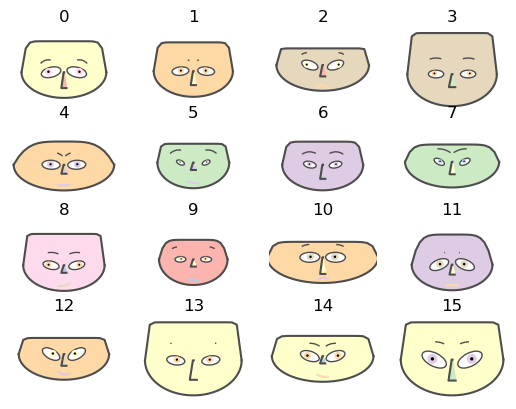
Random data

# Generate data
numpy.random.seed(32)
data = numpy.random.rand(16, 12)

# Make Chernoff faces
fig = chernoff_face(data=data,
                    titles=[str(x) for x in list(range(len(data)))],
                    color_mapper=matplotlib.cm.Pastel1)

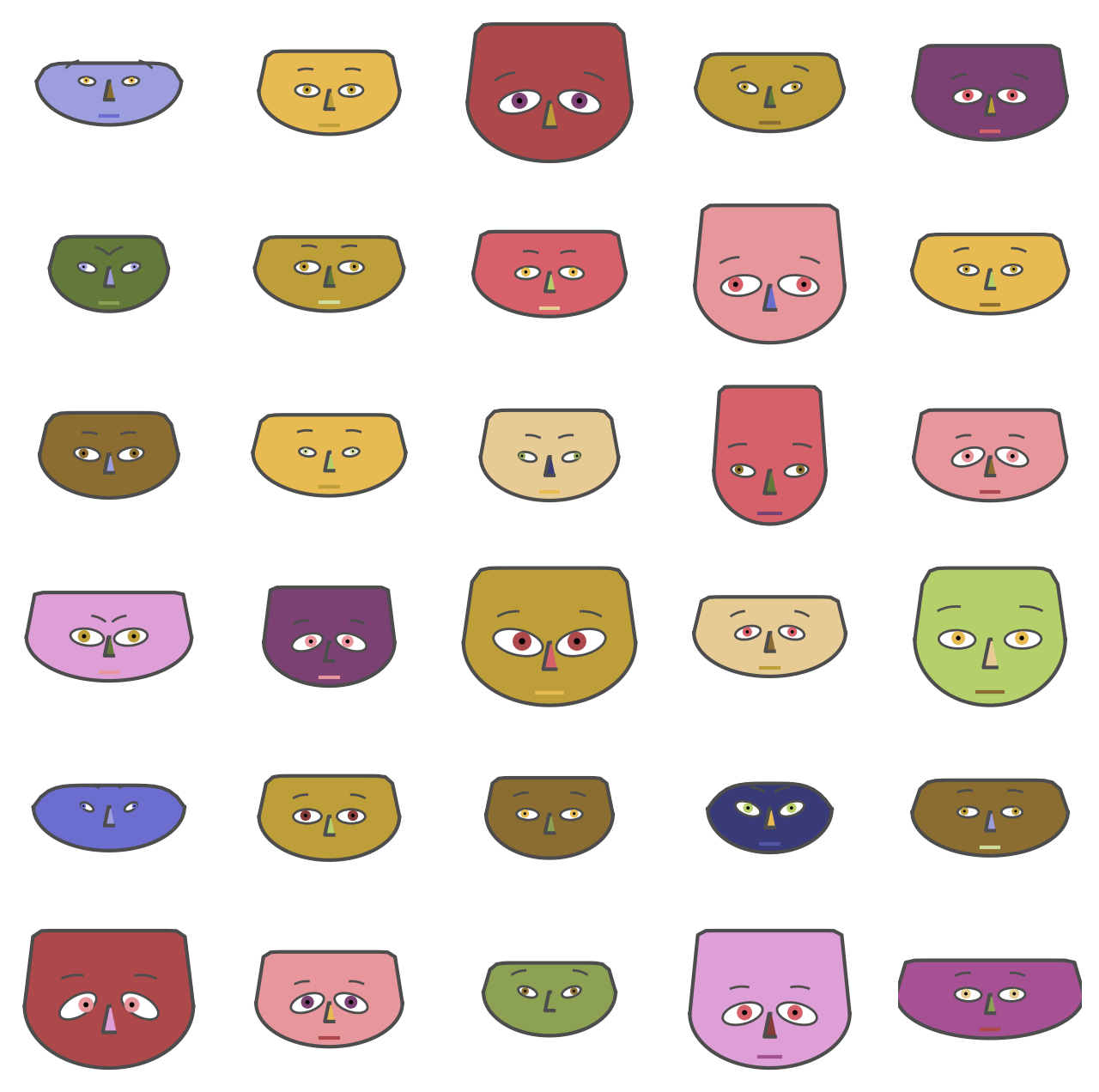
Employee attitude data

Get Employee attitude data

dfData=load_employee_attitude_data_frame()
dfData.head()

	Rating	Complaints	Privileges	Learning	Raises	Critical	Advancement
0	43	51	30	39	61	92	45
1	63	64	51	54	63	73	47
2	71	70	68	69	76	86	48
3	61	63	45	47	54	84	35
4	81	78	56	66	71	83	47

Rescale the variables:

dfData2 = variables_rescale(dfData)
dfData2.head()

	Rating	Complaints	Privileges	Learning	Raises	Critical	Advancement
0	0.066667	0.264151	0.000000	0.121951	0.400000	1.000000	0.425532
1	0.511111	0.509434	0.396226	0.487805	0.444444	0.558140	0.468085
2	0.688889	0.622642	0.716981	0.853659	0.733333	0.860465	0.489362
3	0.466667	0.490566	0.283019	0.317073	0.244444	0.813953	0.212766
4	0.911111	0.773585	0.490566	0.780488	0.622222	0.790698	0.468085

Make the corresponding Chernoff faces:

fig = chernoff_face(data=dfData2,
                    n_columns=5,
                    long_face=False,
                    color_mapper=matplotlib.cm.tab20b,
                    figsize=(8, 8), dpi=200)

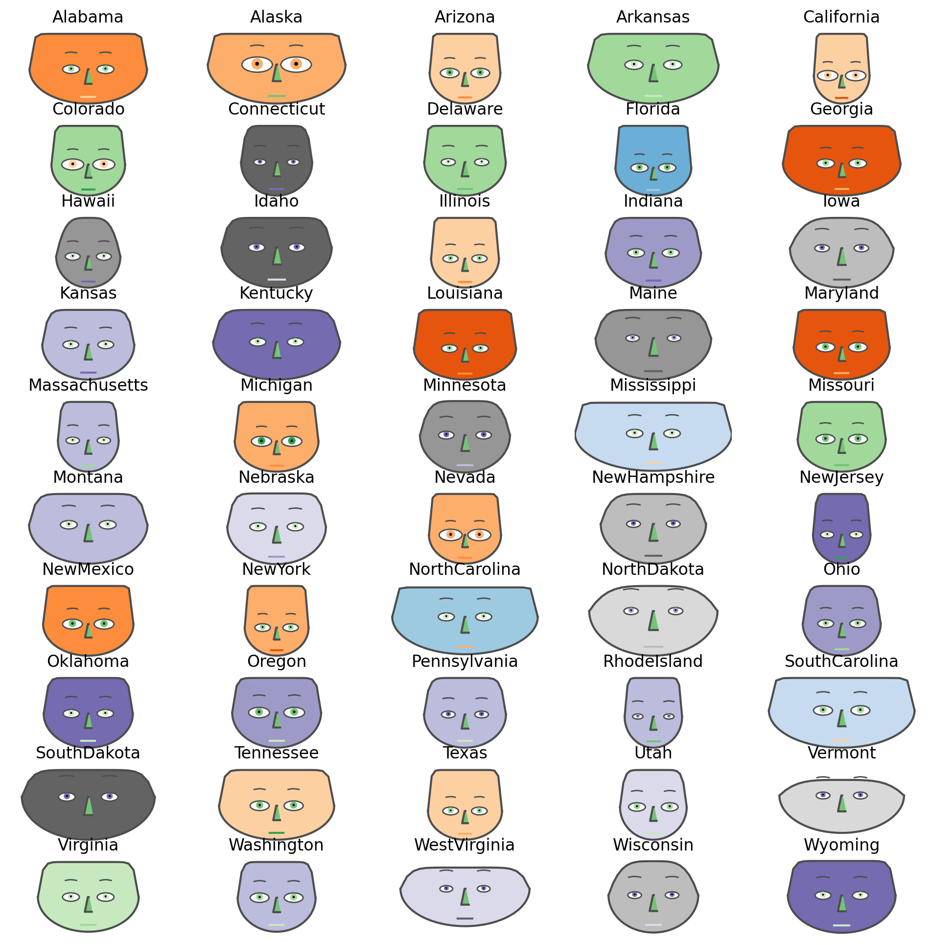
USA arrests data

Get USA arrests data:

dfData=load_usa_arrests_data_frame()
dfData.head()

	StateName	Murder	Assault	UrbanPopulation	Rape
0	Alabama	13.2	236	58	21.2
1	Alaska	10.0	263	48	44.5
2	Arizona	8.1	294	80	31.0
3	Arkansas	8.8	190	50	19.5
4	California	9.0	276	91	40.6

Rescale the variables:

dfData2 = variables_rescale(dfData)
dfData2.head()

	StateName	Murder	Assault	UrbanPopulation	Rape
0	Alabama	0.746988	0.654110	0.440678	0.359173
1	Alaska	0.554217	0.746575	0.271186	0.961240
2	Arizona	0.439759	0.852740	0.813559	0.612403
3	Arkansas	0.481928	0.496575	0.305085	0.315245
4	California	0.493976	0.791096	1.000000	0.860465

Make the corresponding Chernoff faces using USA state names as titles:

fig = chernoff_face(data=dfData2,
                    n_columns=5,
                    long_face=False,
                    color_mapper=matplotlib.cm.tab20c_r,
                    figsize=(12, 12), dpi=200)

---

References

Articles

[AA1] Anton Antonov, “Making Chernoff faces for data visualization”, (2016), MathematicaForPrediction at WordPress.

Functions and packages

[AAf1] Anton Antonov, ChernoffFace, (2019), Wolfram Function Repository.

[AAp1] Anton Antonov, Chernoff faces implementation in Mathematica, (2016), MathematicaForPrediction at GitHub.